Earthquake Data Preparation & Analysis
- Project Purpose
- Final Output
- GitHub Repository Link
- Data Source
- Dataset Information
- 1. Initial Data Exploration
- 2. Collect, Explore and Transform data using R script
- 3. Data Exploration
- 4. Create Reporting Dashboards using Tableau
Project Purpose
The purpose of this project is to collect, explore, and transform data using R programming language, to make it ready for creating reporting dashboards in Tableau.
Final Output
A CSV file with 1,056,144 records and 9 columns of earthquakes data from January 2013 to April 2023 with magnitude 1 and above.
GitHub Repository Link
The source code for this project can be found at my GitHub Repository
Data Source
The earthquake data for this project is collected from the USGS Earthquake Hazards Program website. There are multiple ways to collect data from their website. They have search catalog, web service API, and wrapper libraries for a few programming languages. The search result limit is 20,000 records. For this project, I want to collect the data from January 2013 to April 2023, so using either web service API or wrapper library would be a suitable choice.
I am going to use the Web Service API, and use count and query methods to check records count and to download earthquake data.
If anyone is interested, below are the alternative ways to collect data.
- The data can manually be searched and downloaded by using the Search Earthquake Catalog webpage.
- They also have ComCat Wrapper Libraries and Demonstration Code for Python, R, and Matlab.
Dataset Information
The USGS monitors and reports on earthquakes, assesses earthquake impacts and hazards, and conducts targeted research on the causes and effects of earthquakes.
The variables and their data types, typical values and descriptions are documented at
ANSS Comprehensive Earthquake Catalog (ComCat) Documentation. The full comprehensive documentation can be found here.
1. Initial Data Exploration
To understand the data better before writing the script, we will start by exploring the data using the R console.
1.1 Check the total records to be downloaded
Since the purpose is to download the data from 2013 to 2023, it’s better to check how many records in total that would be. We use the count method of web service API to get that number. First, we need to load the package httr to use HTTP verbs. Then, we use GET() function to get response of a given URL and content() function to get the number. In the URL, starttime, endtime and minmagnitued are user-defined parameters. starttime is set as 2013-01-0100:00:00, endtime is set as 2023-05-1623:59:59 and minmagnitued is set as 1. The starttime and endtime use yyyy-mm-ddhh:mm:ss format.
library(httr)
content(GET("https://earthquake.usgs.gov/fdsnws/event/1/count?starttime=2013-01-0100:00:00&endtime=2023-05-1623:59:59&minmagnitude=1"))
The returned value – 1,059,129, is the total number of records to be downloaded. The download limit is 20,000 records per file, so we will need to separate the data to download into multiple files.
[1] "1059129"
To get the idea of how many records a month could have, we pick a random month, January 2019, and call the API.
content(GET("https://earthquake.usgs.gov/fdsnws/event/1/count?starttime=2019-01-0100:00:00&endtime=2019-01-3123:59:59&minmagnitude=1"))
The returned value – 7,963, is the total number of records to be downloaded for January 2019. In this case, the records count is within the 20,000 result limit. So, we will most likely be able to download the files per month.
[1] "7963"
1.2 Download sample data
After checking the records count, we should start checking the data to get the idea of what kind of data we are dealing with. For this, we can download a small portion of data and explore it. To download the data in a CSV file format, we use download.file() function. The URL of the query method of web service API along with starttime, endtime and minmagnitued parameters, destination file name and extension, and the download method are given as arguments.
download.file("https://earthquake.usgs.gov/fdsnws/event/1/query?format=csv&starttime=2019-01-0100:00:00&endtime=2019-01-3123:59:59&minmagnitude=1", destfile = "sample_data.csv", method = "curl")
The data is downloaded in the CSV file format. The download information is displayed in the console.
  % Total    % Received % Xferd  Average Speed   Time    Time     Time  Current
                                 Dload  Upload   Total   Spent    Left  Speed
100 1393k    0 1393k    0     0   694k      0 --:--:--  0:00:02 --:--:--  695k
1.3 Explore sample data
Now that we have downloaded the file, we can start reading the data. To do that, we use read_csv() function of readr package and give the file name as an argument.
library(readr)
sample_data <- read_csv("sample_data.csv")
The sample_data data frame is created with the table format. The numbers of rows (observations) and columns (variables) created is displayed. In this case, 7,963 rows and 22 columns. Column specification is displayed as summary as well. Here, we can see the data type and the column names. There are 8 columns with character data type, 12 columns with double data type, and 2 columns with datetime data type.
Rows: 7963 Columns: 22
── Column specification ───────────────────────────────────────────────────────
Delimiter: ","
chr   (8): magType, net, id, place, type, status, locationSource, magSource
dbl  (12): latitude, longitude, depth, mag, nst, gap, dmin, rms, horizontalError, depthError, magError, magNst
dttm  (2): time, updated

ℹ Use `spec()` to retrieve the full column specification for this data.
ℹ Specify the column types or set `show_col_types = FALSE` to quiet this message.
To see the full specification with some data, I prefer to use str() function. It compactly displays the internal structure of an R object. So, we can view most of the information neatly.
str(sample_data)
We can easily see that there are NA values in some columns, the place column has both the approximate location and country information, and that some columns such as locationSource and magSource will not be necessary for our reporting dashboard.
spc_tbl_ [7,963 × 22] (S3: spec_tbl_df/tbl_df/tbl/data.frame)
 $ time           : POSIXct[1:7963], format: "2019-01-31 23:53:56" "2019-01-31 23:36:43" "2019-01-31 23:26:59" "2019-01-31 23:14:45" ...
 $ latitude       : num [1:7963] 59.5 61.4 58 61.5 18 ...
 $ longitude      : num [1:7963] -151.2 -150 -153.5 -150 -66.9 ...
 $ depth          : num [1:7963] 9.2 44 59.7 44.7 13 43.7 2.27 77 67.5 35 ...
 $ mag            : num [1:7963] 1.3 1.5 1.6 1 1.65 2.5 1.7 2.97 1.4 4.5 ...
 $ magType        : chr [1:7963] "ml" "ml" "ml" "ml" ...
 $ nst            : num [1:7963] NA NA NA NA 3 NA 13 3 NA NA ...
 $ gap            : num [1:7963] NA NA NA NA 253 NA 57 259 NA 159 ...
 $ dmin           : num [1:7963] NA NA NA NA 0.108 ...
 $ rms            : num [1:7963] 0.34 0.42 0.53 0.36 0.45 0.94 0.09 0.16 0.55 0.41 ...
 $ net            : chr [1:7963] "ak" "ak" "aacse" "ak" ...
 $ id             : chr [1:7963] "ak0191fno7bz" "ak0191fnkjco" "aacse0191fnifdr" "ak0191fnftsr" ...
 $ updated        : POSIXct[1:7963], format: "2019-02-15 22:29:46" "2019-02-15 22:29:45" "2021-05-21 15:46:36" "2019-02-15 22:29:45" ...
 $ place          : chr [1:7963] "10 km S of Halibut Cove, Alaska" "8 km SSW of Big Lake, Alaska" "37 km W of Aleneva, Alaska" "Southern Alaska" ...
 $ type           : chr [1:7963] "earthquake" "earthquake" "earthquake" "earthquake" ...
 $ horizontalError: num [1:7963] NA NA NA NA 5.79 NA 0.39 8.21 NA 8.2 ...
 $ depthError     : num [1:7963] 0.2 0.2 0.2 0.4 7.37 ...
 $ magError       : num [1:7963] NA NA NA NA 0.08 NA 0.12 0.1 NA 0.163 ...
 $ magNst         : num [1:7963] NA NA NA NA 2 NA 4 3 NA 11 ...
 $ status         : chr [1:7963] "reviewed" "reviewed" "reviewed" "reviewed" ...
 $ locationSource : chr [1:7963] "ak" "ak" "aacse" "ak" ...
 $ magSource      : chr [1:7963] "ak" "ak" "aacse" "ak" ...
 - attr(*, "spec")=
  .. cols(
  ..   time = col_datetime(format = ""),
  ..   latitude = col_double(),
  ..   longitude = col_double(),
  ..   depth = col_double(),
  ..   mag = col_double(),
  ..   magType = col_character(),
  ..   nst = col_double(),
  ..   gap = col_double(),
  ..   dmin = col_double(),
  ..   rms = col_double(),
  ..   net = col_character(),
  ..   id = col_character(),
  ..   updated = col_datetime(format = ""),
  ..   place = col_character(),
  ..   type = col_character(),
  ..   horizontalError = col_double(),
  ..   depthError = col_double(),
  ..   magError = col_double(),
  ..   magNst = col_double(),
  ..   status = col_character(),
  ..   locationSource = col_character(),
  ..   magSource = col_character()
  .. )
 - attr(*, "problems")=<externalptr>
After str(), I use summary() function to see the summary statistics. It helps to understand the numerical data better, as well as see the total number of NA values in each column.
summary(sample_data)
      time                           latitude
 Min.   :2019-01-01 00:04:00.75   Min.   :-64.94
 1st Qu.:2019-01-08 14:16:24.94   1st Qu.: 33.23
 Median :2019-01-15 21:04:25.75   Median : 46.87
 Mean   :2019-01-16 05:48:41.27   Mean   : 41.92
 3rd Qu.:2019-01-23 15:21:38.52   3rd Qu.: 61.41
 Max.   :2019-01-31 23:53:56.27   Max.   : 85.85

   longitude          depth              mag
 Min.   :-179.9   Min.   : -3.480   Min.   :1.000
 1st Qu.:-150.2   1st Qu.:  6.995   1st Qu.:1.300
 Median :-144.6   Median : 15.640   Median :1.700
 Mean   :-108.7   Mean   : 38.999   Mean   :2.149
 3rd Qu.:-115.5   3rd Qu.: 43.900   3rd Qu.:2.570
 Max.   : 180.0   Max.   :623.950   Max.   :6.800

   magType               nst             gap
 Length:7963        Min.   :  0.0   Min.   : 11.0
 Class :character   1st Qu.: 10.0   1st Qu.: 68.0
 Mode  :character   Median : 18.0   Median :104.0
                    Mean   : 23.5   Mean   :123.7
                    3rd Qu.: 33.0   3rd Qu.:161.9
                    Max.   :221.0   Max.   :355.5
                    NA's   :5134    NA's   :3626
      dmin             rms             net
 Min.   : 0.000   Min.   :0.0000   Length:7963
 1st Qu.: 0.047   1st Qu.:0.1900   Class :character
 Median : 0.175   Median :0.4300   Mode  :character
 Mean   : 1.153   Mean   :0.4498
 3rd Qu.: 1.268   3rd Qu.:0.6200
 Max.   :36.335   Max.   :2.9400
 NA's   :3736
      id               updated
 Length:7963        Min.   :2019-01-01 01:35:02.50
 Class :character   1st Qu.:2019-01-17 18:50:06.83
 Mode  :character   Median :2019-01-29 21:12:18.36
                    Mean   :2019-04-10 09:43:53.80
                    3rd Qu.:2019-04-02 20:52:06.03
                    Max.   :2023-04-01 03:09:54.75

    place               type           horizontalError
 Length:7963        Length:7963        Min.   : 0.090
 Class :character   Class :character   1st Qu.: 0.300
 Mode  :character   Mode  :character   Median : 0.980
                                       Mean   : 3.619
                                       3rd Qu.: 6.600
                                       Max.   :31.200
                                       NA's   :3907
   depthError         magError         magNst
 Min.   :  0.000   Min.   :0.000   Min.   :  0.00
 1st Qu.:  0.300   1st Qu.:0.100   1st Qu.:  6.00
 Median :  0.600   Median :0.150   Median : 14.00
 Mean   :  2.701   Mean   :0.180   Mean   : 22.39
 3rd Qu.:  1.920   3rd Qu.:0.215   3rd Qu.: 25.00
 Max.   :132.200   Max.   :5.410   Max.   :582.00
                   NA's   :3765    NA's   :3722
    status          locationSource      magSource
 Length:7963        Length:7963        Length:7963
 Class :character   Class :character   Class :character
 Mode  :character   Mode  :character   Mode  :character
Another way to view only the NA values count is to use is.na() function together with colSums() function.
colSums(is.na(sample_data))
           time        latitude       longitude           depth
              0               0               0               0
            mag         magType             nst             gap
              0               0            5134            3626
           dmin             rms             net              id
           3736               0               0               0
        updated           place            type horizontalError
              0               0               0            3907
     depthError        magError          magNst          status
              0            3765            3722               0
 locationSource       magSource
              0               0
Now that we have got a good overview of our data, we should also check if there are any duplicated rows. We use duplicated() function for this purpose.
sample_data[duplicated(sample_data),]
Since we have a tibble with 0 rows (observations), it means that we don’t have any duplicated rows. Now that we have a good understanding of our data structure, we can start with writing a script.
# A tibble: 0 × 22
# … with 22 variables: time <dttm>, latitude <dbl>, longitude <dbl>, depth <dbl>, mag <dbl>, magType <chr>, nst <dbl>, gap <dbl>, dmin <dbl>, rms <dbl>, net <chr>,
#   id <chr>, updated <dttm>, place <chr>, type <chr>, horizontalError <dbl>, depthError <dbl>, magError <dbl>, magNst <dbl>, status <chr>, locationSource <chr>,
#   magSource <chr>
# ℹ Use `colnames()` to see all variable names
2. Collect, Explore and Transform data using R script
In this part of the project, R script is created to:
- access web service API and query the data,
- download the result files,
- merge the downloaded files,
- explore and clean the merged data to make it ready for the reporting dashboard, and
- create a CSV file with the final tidy data.
httr, lubridate, readr, dplyr, tidyr, and stringr packages are used to collect and manipulate data. The GET() function of httr package is used to access the web service API to get a response from the count function to query the total number of results. readr package is used to read csv file into a data frame. lubridate package is used to turn data into date data type and to manipulate dates. dplyr, tidyr, and stringr packages are used to manipulate and tidy data.
First, import necessary packages to use their functions.
library(httr)
library(lubridate)
library(readr)
library(dplyr)
library(tidyr)
library(stringr)
Set the working directory as the source file directory. So that when the files are downloaded, they will be downloaded to the same directory as the R script file. If you use RStudio to run this code, you will get an error message. In that case, you can comment out this code.
setwd(getSrcDirectory(function(){})[1])
The files are to be downloaded to a folder named ‘EQData’. The file_path variable is declared in a global environment so that it can be used from anywhere. If there is a need to change the download folder name, it can be edited here.
file_path <- "./EQData"
After the file_path is declared, we check if the folder ‘EQData’ already existed or not by using dir.exists() function and giving file_path as an argument. Here, we only need to create a new folder if it does not exist. So, ! keyword is used to check if the folder does not exist. If it does not, we create a new folder by using dir.create() function and giving file_path as an argument.
# Check if the folder exists, if not, create one.
if (!dir.exists(file_path)) {
  dir.create(file_path)
}
To query the data using the web service API, we need to pass start date and end date parameters. We need to make sure that the data passed are in date data type, and that the end date is not earlier than the start date. The ValidateDates() function validates the dates and stops the script if a validation failed. The first validation used is.Date() function from lubridate package, together with ! keyword, to check if either of the startDate and endDate arguments are not in date data type. If either one are not in date data type, we need the script to stop running and show an error message. To achieve that, we use stop() function execution with an appropriate error message. For the second validation, we just need to check if the endDate is earlier than the startDate. Then, use stop() function again with an appropriate error message. This function can be called whenever we need to validate the start date and the end date.
ValidateDates <- function(startDate, endDate) {
  # Validates the start and end date range arguments and shows stop message if
  # one of the validations failed.
  # Validation 1: Check if the given arguments are not valid dates.
  # Validation 2: Check if the End Date is earlier than the Start Date.
  #
  # Args:
  #    startDate (Date): Start Date parameter of the query.
  #    endDate (Date): End Date parameter of the query.
  #
  # Returns:
  #    No return value.

  # Check if the given arguments are not valid dates.
  if (!is.Date(startDate) | !is.Date(endDate)) {
    stop("Please give valid date parameters using as.Date or as_date
         functions.")
  }
  # Check if the End Date is earlier than the Start Date.
  else if (endDate < startDate) {
    stop("End Date must be later than the Start Date.")
  }
}
Before we download the records, we need to make sure that the records count to download does not exceed 20,000 records. We can call the count method of web service API to get the total number of records. We will be checking the records count every time we download a file for each month. Below function will first validate the startDate and endDate arguments by calling ValidateDates() function. Then, the API URL of count method is concatenated and called using the given arguments. From the response, we get the number of records by using content() function. Since the response returned is in character data type, as.integer() function is used to change it to integer data type and return the value.
CheckRecordsCount <- function(startDate, endDate) {
  # Queries the record count to be downloaded for the given date arguments.
  #
  # Args:
  #    startDate (Date): Start Date parameter of the query.
  #    endDate (Date): End Date parameter of the query.
  #
  # Returns:
  #    The total number of records. Integer data type.

  # Validate date arguments.
  ValidateDates(startDate, endDate)

  records_num_url <-
    GET(
      paste0(
        "https://earthquake.usgs.gov/fdsnws/event/1/count?starttime=",
        startDate,
        "00:00:00&endtime=",
        endDate,
        "23:59:59",
        "&minmagnitude=1"
      )
    )
  total_records <- as.integer(content(records_num_url))
  return(total_records)
}
For the files to be downloaded, the file names should be in a format that is easy to keep track of. We will be using the file name format as text_yyyy_mmm.extension, “earthquake_data_2013_Jan.csv”. So, following function gets the fileDate and fileExtension arguments and concatenate them together with file_path variable to get a file name. The file name is returned as a character value.
SetFileName <- function(fileDate, fileExtension) {
  # Sets a file name to be saved as for the file to download.
  #
  # Args:
  #    fileDate (Date): File Date to get month and year.
  #    fileExtension (character): File extension to be saved as.
  #
  # Returns:
  #    A file name to be saved as. character data type.

  file_name <-
    paste0(
      file_path,
      "/earthquake_data_",
      year(fileDate),
      "_",
      month(fileDate, label = TRUE),
      fileExtension
    )

  return(file_name)
}
The DownloadFile() function gets the startDate, endDate, and fileName arguments and downloads the query results. Before downloading the file, ValidateDates() function is called to validate the given dates. Then, the API URL of query method is concatenated using the given arguments. After concatenating the URL, we use download.file() function to download a CSV file by passing the API URL, given file name, and download method. A CSV file will be downloaded to the destination folder.
DownloadFile <- function(startDate, endDate, fileName) {
  # Downloads the query results as a csv file using the query URL.
  #
  # Args:
  #    startDate (Date): Start Date parameter of the query.
  #    endDate (Date): End Date parameter of the query.
  #    fileName (character): File name to be saved as, including path and
  #              extension.
  #
  # Returns:
  #    No return value.

  # Validate date arguments.
  ValidateDates(startDate, endDate)

  file_url <-
    paste0(
      "https://earthquake.usgs.gov/fdsnws/event/1/query?format=csv&starttime=",
      startDate,
      "00:00:00&endtime=",
      endDate,
      "23:59:59",
      "&minmagnitude=1"
    )
  download.file(file_url, destfile = fileName, method = "curl")
}
The DownloadFile() function above downloads a file, usually for a particular month, while the DownloadAll() function below prepares and processes the download of all files for all the months between the given startDate and endDate arguments. The startDate and the endDate arguments set the date range that needs to be downloaded. First, ValidateDates() function is called to validate the given date arguments. To download for all the months between the given startDate and endDate, the while() loop is used together with a stop flag variable to iterate for the file download of each month, until the endDate is reached.
For the file download, the result records limit is 20,000 per download. So, for easier tracking, the file is downloaded per month using iteration. If per month still exceeds 20,000 records, the records for that month are separated into three files. 10 days each for the first two files and the remaining days in the last file. Separating the data into three files helps us ensure that the result limit will not be exceeded. So, to download the files for each month, we need to use a date range for that particular month. We cannot use startDate and endDate arguments. The curr_start_date and the curr_end_date variables are used to set the start date and the end date of the current month to download. For the first download, curr_start_date is set with the value of startDate argument, and the curr_end_date is set by using the ceiling_date() function of lubridate package to get the last day of the month. The curr_end_date variable is then validated against endDate to ensure that it is not later than the endDate. If it is, the curr_end_date variable is set with the value of endDate, and the last_dl flag is set as TRUE. By reaching the endDate, the download is done, and the next iteration will be stopped. If the endDate is not reached yet, the iteration will continue, and in the next iteration, a day is added to the curr_end_date variable and set it as the value of the curr_start_date variable. That way, we will download the file for the next month and the iteration will continue until the endDate is reached.
After the values of the curr_start_date and the curr_end_date are defined, we call the CheckRecordsCount() function with the curr_start_date and the curr_end_date as arguments. Then, we validate if the records_to_dl value is more than 20,000 records. If it is more than the limit, we separate the date range into 10 days each in the first two files and the remaining days in the last file. The file_ext variable is used to concatenate “-1”, “-2”, or “-3” before the given fileExtension value. The SetFileName() function is called with the arguments curr_start_date and file_ext, then, set the returned file name value to the file_name variable. After setting the file name, we call DownloadFile() function. The arguments given to the function varied for each file.
- For the first file, to download the first 10 days, we start the date range from the
curr_start_dateand add 9 days to get the end date. So, the arguments given are:curr_start_date,curr_start_date + days(9), andfile_name. - For the second file, to download the next 10 days, we start the date range from the day 11 to the day 20. So, the arguments given are:
curr_start_date + days(10),curr_start_date + days(19), andfile_name. - For the last file, to download the last remaining days, we start the date range from the day 21 to the last day of the month. So, the arguments given are:
curr_start_date + days(20),curr_end_date, andfile_name. For the months with less than 20,000 results, we callDownloadFile()function with the argumentscurr_start_date,curr_end_dateandfile_name. Then, we add the number of records downloaded to thedownloaded_recordsvariable, to keep track of the total downloaded records. The iteration countitr_countvariable is also incremented to record the total number of iterations.
Lastly, we return the download successful message, including the total number of downloaded records and the number of iterations.
DownloadAll <- function(startDate, endDate, fileExtension) {
  # Prepares to download csv files per month using the given date arguments.
  #
  # Args:
  #    startDate (Date): Start Date parameter of the query.
  #    endDate (Date): End Date parameter of the query.
  #    fileExtension (character): File extension to be saved as.
  #
  # Returns:
  #    A success message. character data type.

  # Validate date parameters.
  ValidateDates(startDate, endDate)

  # define count of records to download for each iteration
  records_to_dl <- 0

  # define count of all downloaded records
  downloaded_records <- 0

  # define iteration count
  itr_count <- 0

  # define iteration stop flag
  last_dl <- FALSE

  # For the file download, the result records limit is 20,000 per download.
  # So, for easier tracking, the file is downloaded per month using iteration.
  # If per month still exceeds 20,000 records, the records for that month are
  # separated into three files download. 10 days each for the first two files and the
  # remaining days in the last file.
  while (last_dl == FALSE) {  # iterate until the flag is set as TRUE.
    # The logic for setting curr_start_date is to check the iteration count.
    # If it's the 1st iteration, the given startDate argument is used.
    # If it's not the 1st iteration, the value is set by adding one day to the
    # previous iteration's End Date, curr_end_date.
    if (itr_count < 1) {
      curr_start_date <- startDate
    } else {
      curr_start_date <- curr_end_date + days(1)
    }

    # curr_end_date is set as the last day of the month from curr_start_date
    # and validate against the given endDate argument to check if it's later
    # than the endDate. If it is, the curr_end_date is set with the value of
    # endDate argument.
    curr_end_date <- ceiling_date(curr_start_date, "month") %m-% days(1)

    if (curr_end_date >= endDate) {
      curr_end_date <- endDate  # Set as the given argument.
      last_dl <- TRUE  # Set the flag as TRUE to end the iteration.
    }

    # Check the current record counts to be downloaded.
    records_to_dl <- CheckRecordsCount(curr_start_date, curr_end_date)

    # Check if the record limit is exceeded, if true, separate as three files.
    # If not, download the records.
    if (records_to_dl > 20000) {
      # Set file name of the 1st file to be saved as.
      file_ext <- paste0("-1", fileExtension)
      file_name <- SetFileName(curr_start_date, file_ext)

      # Download the first 10 days.
      DownloadFile(curr_start_date, curr_start_date + days(9), file_name)

      # Set file name of the 2nd file to be saved as.
      file_ext <- paste0("-2", fileExtension)
      file_name <- SetFileName(curr_start_date, file_ext)

      # Download another 10 days.
      DownloadFile(curr_start_date + days(10), curr_start_date + days(19), file_name)

      # Set file name of the last file to be saved as.
      file_ext <- paste0("-3", fileExtension)
      file_name <- SetFileName(curr_start_date, file_ext)

      # Download the remaining days.
      DownloadFile(curr_start_date + days(20), curr_end_date, file_name)

    } else {
      # Set file name of the last file to be saved as.
      file_name <- SetFileName(curr_start_date, fileExtension)

      # Download the file for the month.
      DownloadFile(curr_start_date, curr_end_date, file_name)
    }
    # Increment the downloaded records.
    downloaded_records <- downloaded_records + records_to_dl
    # Increment the iteration count.
    itr_count <- itr_count + 1
  }

  # Return the success message.
  return(
    paste0(
      "Successfully downloaded ",
      downloaded_records,
      " records in ",
      itr_count,
      " files."
    )
  )
}
After all the files are downloaded, we can start with the file merge. The MergeFiles() function uses the pipe function %>% from dplyr package to chain a few functions in a series. First, the list.files() function is used to list all the files in the given directory, which is the value of global variable file_path. Then, the lapply() function is used to apply read_csv() function to all the files. The bind_rows() function is applied last to bind the records of the all the files read. The merged data frame is returned.
MergeFiles <- function() {
  # Reads all the files in the given directory and bind them by rows.
  #
  # Args:
  #    None.
  #
  # Returns:
  #    A data frame of merged rows.

  eqk_data <- list.files(path = file_path, full.names = TRUE) %>%
    lapply(read_csv) %>%
    bind_rows()

  return(eqk_data)
}
We now have a merged data frame with all the records. Referring to the sample data we explored in section 1.3 Explore sample data, we can now start cleaning the data. The RemoveDuplicates() function removes all the duplicated rows if exist. Most functions used here are from the dplyr package. The pipe function %>% is used to apply the group_by_all() function to group the records. Then, the filter() function used to filter the groups with more than 1 records (i.e. duplicated rows). The ungroup() function is applied last to ungroup the data. So, we get duplicated rows in a data frame. The nrow() function is used to check if there is any record. If there is, the distinct() function is used to filter only the unique records. The unique data frame is then returned. The advantage of checking the duplicated records this way is that we have the data frame of duplicated records if we want to view the data. Otherwise, we can skip everything and just use the line df <- distinct(df) to get the unique records.
RemoveDuplicates <- function(df) {
  # Removes all the duplicated rows.
  #
  # Args:
  #    df (data frame): A data frame to remove duplicates.
  #
  # Returns:
  #    A data frame of unique rows.

  # Check if duplicated rows exists
  duplicate_rows <- df %>%
    group_by_all() %>%
    filter(n() > 1) %>%
    ungroup()

  # Remove duplicates if there is any
  if (nrow(duplicate_rows) > 0) {
    df <- distinct(df)
  }

  return(df)
}
The CheckMissingDates() function checks and returns all the missing dates from the data frame, within the range of given date arguments. First, we convert the time column as date data type using as.Date() function. Then, we generate a list of all dates between the given startDate and endDate arguments using seq() function. After that, we filter the dates from the all_dates which are not in the given data frame argument. They are the missing dates in the given data frame and the result is returned.
CheckMissingDates <- function(df, startDate, endDate) {
  # Returns all the missing dates from the data frame between the start date and
  # the end date. If there is a missing date, it is most likely that the
  # downloaded files were incomplete.
  #
  # Args:
  #    df (data frame): A data frame to check the missing dates.
  #    startDate (Date): Start Date parameter to check the missing dates.
  #    endDate (Date): End Date parameter to check the missing dates.
  #
  # Returns:
  #    A list of missing dates.

  # Convert time column as Date data type.
  df$time <- as.Date(df$time)

  # Get a list of all dates within the given start and end dates in sequence.
  all_dates <- seq(startDate, endDate, by = 1)

  # Check if there is any date from all_dates that are not in df.
  missing_dates <- all_dates[!all_dates %in% df$time]

  return(missing_dates)
}
The SeparateLocationColumn() function separates place column into two columns, Location Detail and Location. When exploring the sample data, we saw that the place column contains the approximate location and the country name separated by commas. We only need the country name information. The country name is after the last comma. So, we need to make sure that we use the last comma as a separator to get the country names only. We use separate() function from tidyr package to separate the column. A regular expression- ,(?=[^,]*$) is used to match the last comma as a separator. To understand the regular expression, test it out at RegExr website. The data frame with separated columns is returned.
SeparateLocationColumn <- function(df) {
  # Separates 'place' column into two columns: 'Location Detail' and 'Location'.
  # The last comma is used as a separator.
  #
  # Args:
  #    df (data frame): A data frame to check the missing dates.
  #
  # Returns:
  #    A data frame with separated columns.

  df_separated <-
    separate(
      data = df,
      col = "place",
      into = c("Location Detail", "Location"),
      sep = ",(?=[^,]*$)"
    )

  return(df_separated)
}
The CleanData() function cleans the Location column by trimming extra spaces and setting title case. It also drops the records with NA in location, latitude, longitude columns, and replaces the US States abbreviations with names. The functions from tidyr, stringr, and dplyr packages are used. The cleaned data frame is returned.
CleanData <- function(df) {
  # Cleans the Location column by trimming extra spaces and setting title case.
  # Drops the records with NA in location, latitude, longitude columns.
  # Replaces the abbreviations.
  #
  # Args:
  #    df (data frame): A data frame to clean the data.
  #
  # Returns:
  #    A data frame with a cleaned data.

  df_cleaned <- df %>%
    mutate(
      Location = case_when(is.na(Location) ~ `Location Detail`,
                           TRUE ~ Location) %>%
        str_trim(.) %>%
        str_to_title(.) %>%
        # A named vector is used to match multiple patterns.
        str_replace_all(., c("\\bAk\\b" = "Alaska",
                             "\\bAr\\b" = "Arkansas",
                             "\\bAz\\b" = "Arizona",
                             "\\bCa\\b" = "California",
                             "\\bCo\\b" = "Colorado",
                             "\\bHi\\b" = "Hawaii",
                             "\\bId\\b" = "Idaho",
                             "\\bKs\\b" = "Kansas",
                             "\\bKy\\b" = "Kentucky",
                             "\\bMn\\b" = "Minnesota",
                             "\\bMo\\b" = "Missouri",
                             "\\bMt\\b" = "Montana",
                             "\\bMx\\b" = "Mexico",
                             "\\bNc\\b" = "North Carolina",
                             "\\bNj\\b" = "New Jersey",
                             "\\bNm\\b" = "New Mexico",
                             "\\bNy\\b" = "New York",
                             "\\bNv\\b" = "Nevada",
                             "\\bOk\\b" = "Oklahoma",
                             "\\bOr\\b" = "Oregon",
                             "\\bTn\\b" = "Tennessee",
                             "\\bTx\\b" = "Texas",
                             "\\bUsa\\b" = "USA",
                             "\\bUt\\b" = "Utah",
                             "\\bWa\\b" = "Washington",
                             "\\bWy\\b" = "Wyoming"))
    ) %>%
    drop_na(latitude) %>% # Drop records with latitude as NA
    drop_na(longitude) %>% # Drop records with longitude as NA
    drop_na(Location) # Drop records with Location as NA

  # Drop unnecessary columns
  df_cleaned <- select(df_cleaned, -c(nst, gap, dmin, rms, net, updated, horizontalError, depthError, magError, magNst, status, locationSource, magSource, 'Location Detail'))

  # Get all locations with abbreviations.
  # df_abbr <- df_cleaned$Location[nchar(as.character(df_cleaned$Location)) < 4]

  # Check the unique abbreviations.
  # sort(unique(df_abbr))

  return(df_cleaned)
}
Now that we have a cleaned tidy data, we can create a CSV file. The CreateCSV() function creates a CSV file using the write.csv() function. The file created message is returned.
CreateCSV <- function(df) {
  # Creates a csv file with the merged and cleaned data.
  #
  # Args:
  #    df (data frame): A data frame of cleaned data.
  #
  # Returns:
  #    A file created message.

  write.csv(df, file = "./earthquakes-data.csv", row.names=FALSE)
  return(paste0("File created with name earthquakes-data.csv and contains ",
                nrow(df), " rows and ", ncol(df), " columns."))
}
We have finished writing the functions and we can start calling them with the appropriate arguments. First, start_date, end_date, and file_extension variables are defined. The end_date variable is set as today date using Sys.Date() function. After setting the variables, we call the functions one by one and pass appropriate arguments. Then, we print the file download message, the file create message, and the missing dates message, so that we can see them in the console.
# Set start date and end date of the search query. Use yyyy-mm-dd date format.
start_date <- as_date("2013-01-01")
end_date <- Sys.Date()
file_extension <- ".csv"

# Run the functions without recording time for each one.
total_record <- CheckRecordsCount(start_date, end_date)
download_message <- DownloadFiles(start_date, end_date, file_extension)
df_merged <- MergeFiles()
df_unique <- RemoveDuplicates(df_merged)
missing_dates <- CheckMissingDates(df_merged, start_date, end_date)
df_separated <- SeparateLocationColumn(df_unique)
df_cleaned <- CleanData(df_separated)
create_message <- CreateCSV(df_cleaned)

# Print results to console.
print(download_message)
print(create_message)

if (length(missing_dates) > 0) {
  print("Following are the missing dates: ")
  print(missing_dates)
} else {
  print("There is no missing date.")
}
Before we run the script, we can add timer to record the time it takes to run the script, including the file downloads. We just need to add the line start_time <- proc.time() at the start of the script and the line print(proc.time() - start_time) at the end of the script.
# Set start time to time the running of the whole script. proc_time data type.
start_time <- proc.time()

# Script Here

# Time the running of the whole script. End time.
print(proc.time() - start_time)
Now, we can run the script. After the script is executed completely, we will see the printed messages in the console as follows. The downloaded data is 1,059,267 records in 124 files. After transformation the data, the tidy data contains 1,056,144 records and 9 columns. The user CPU time, which is charged for the execution of user instructions of the calling process, took 137.53 seconds (2.3 mins). The system CPU time, which is charged for execution by the system on behalf of the calling process, took 22.37 seconds (0.4 mins). The elapsed time, which is the actual elapsed time since the process was started, took 797.80 seconds (13.3 mins).
[1] "Successfully downloaded 1059267 records in 124 files."
[1] "File created with name earthquakes-data.csv and contains 1056144 rows and 9 columns."
[1] "There is no missing date."
   user  system elapsed
 137.53   22.37  797.80
3. Data Exploration
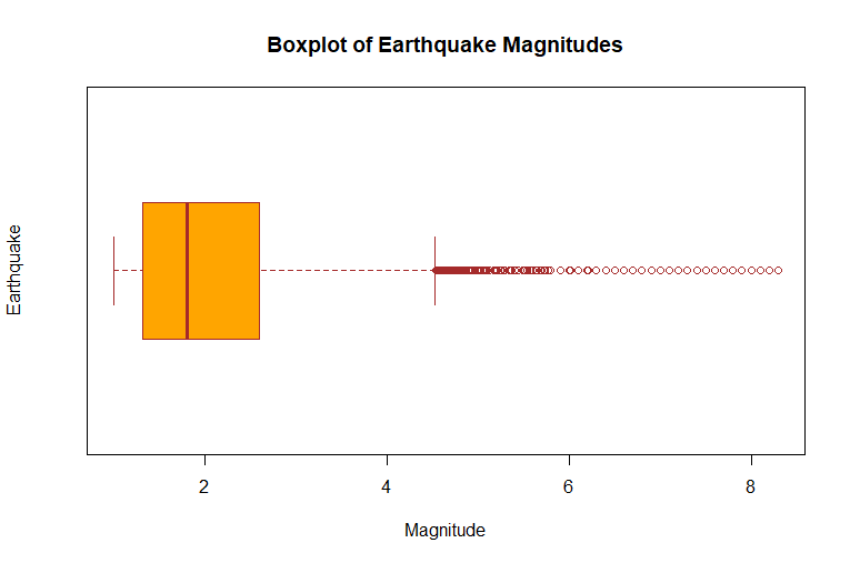
Now that we have a tidy data, we can create a few plots such as boxplot, scatterplot and interactive map to understand the data better.
boxplot(df_cleaned$mag,
        main = "Boxplot of Earthquake Magnitudes",
        xlab = "Magnitude",
        ylab = "Earthquake",
        col = "orange",
        border = "brown",
        horizontal = TRUE
)
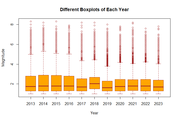
boxplot(mag~year(time),
        data=df_cleaned,
        main="Different Boxplots of Each Year",
        xlab="Year",
        ylab="Magnitude",
        col="orange",
        border="brown"
)
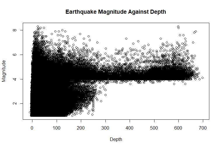
plot(df_cleaned$depth,
     df_cleaned$mag,
     main="Earthquake Magnitude Against Depth",
     xlab="Depth",
     ylab="Magnitude"
)
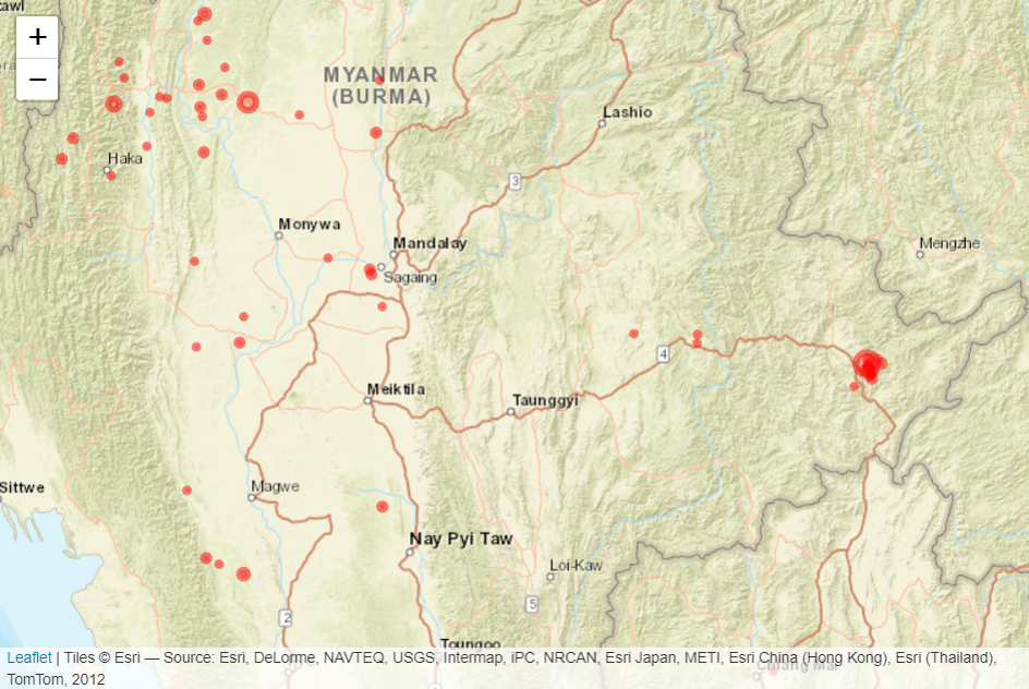
library(leaflet)

# For efficiency, subset only the records of year 2022
df <- df_cleaned[(df_cleaned$time >= "2022-01-01" & df_cleaned$time <= "2022-12-31"),]

leaflet(df) %>%
    addProviderTiles("Esri.WorldStreetMap") %>%
    addCircles(
        lng = ~longitude,
        lat = ~latitude,
        popup = paste0(df$Location, "<br>", df$mag),
        radius = sqrt(10^df$mag) * 10,
        color = "red",
        fillColor = "red",
        fillOpacity = 0.25
    )
4. Create Reporting Dashboards using Tableau
The following Reporting Dashboards are created in Tableau Public. I created the dashboards with fixed width option, so you will need to scroll them horizontally to view everything if you are using a small screen devices such as a laptop. I will create another post on the detailed steps taken to develop these dashboards.